

LLNL Climate and Weather Seminar Series (01/25/2023) - A Gentle Introduction to xCDAT#
“A Python package for simple and robust climate data analysis.”
Core Developers: Tom Vo, Stephen Po-Chedley, Jason Boutte, Jill Zhang, Jiwoo Lee
With thanks to Peter Gleckler, Paul Durack, Karl Taylor, and Chris Golaz
Updated: 03/18/25 [v0.8.0]
This work is performed under the auspices of the U. S. DOE by Lawrence Livermore National Laboratory under contract No. DE-AC52-07NA27344.
Presentation Overview#
Intended audience: Some or no familiarity with xarray and/or xcdat
Driving force behind xCDAT
Goals and milestones of CDAT’s successor
Introducing xCDAT
Understanding the basics of Xarray
How xCDAT extends Xarray for climate data analysis
Technical design philosophy and APIs
Demo of capabilities
How to get involved
Notebook Kernel Setup#
Users can install their own instance of xcdat and follow these examples using their own environment (e.g., with VS Code, Jupyter, Spyder, iPython) or enable xcdat with existing JupyterHub instances.
First, create the conda environment:
conda create -n xcdat_notebook -c conda-forge xcdat xesmf matplotlib ipython ipykernel cartopy nc-time-axis gsw-xarray jupyter pooch
Then install the kernel from the xcdat_notebook environment using ipykernel and name the kernel with the display name (e.g., xcdat_notebook):
python -m ipykernel install --user --name xcdat_notebook --display-name xcdat_notebook
Then to select the kernel xcdat_notebook in Jupyter to use this kernel.
The Driving Force Behind xCDAT#
The CDAT (Community Data Analysis Tools) library has provided a suite of robust and comprehensive open-source climate data analysis and visualization packages for over 20 years
A driving need for a modern successor
Focus on a maintainable and extensible library
Serve the needs of the climate community in the long-term


Goals and Milestones for CDAT’s Successor#
Offer similar core capabilities
For example geospatial averaging, temporal averaging, and regridding
Use modern technologies in the library’s stack
Support parallelism and lazy operations
Be maintainable, extensible, and easy-to-use
Python Enhancement Proposals (PEPs)
Automate DevOps processes (unit testing, code coverage)
Actively maintain documentation
Cultivate an open-source community that can sustain the project
Encourage GitHub contributions
Community engagement efforts (e.g., Pangeo, ESGF)
Introducing xCDAT#
xCDAT is an extension of xarray for climate data analysis on structured grids
Goal of providing features and utilities for simple and robust analysis of climate data
Jointly developed by scientists and developers from:
E3SM Project (Energy Exascale Earth System Model Project)
PCMDI (Program for Climate Model Diagnosis and Intercomparison)
SEATS Project (Simplifying ESM Analysis Through Standards Project)
Users around the world via GitHub



Before We Dive Deeper, Let’s Talk About Xarray#
Xarray is an evolution of an internal tool developed at The Climate Corporation
Released as open source in May 2014
NumFocus fiscally sponsored project since August 2018


Key Features and Capabilities in Xarray#
“N-D labeled arrays and datasets in Python”
Built upon and extends NumPy and pandas
Interoperable with scientific Python ecosystem including NumPy, Dask, Pandas, and Matplotlib
Supports file I/O, indexing and selecting, interpolating, grouping, aggregating, parallelism (Dask), plotting (matplotlib wrapper)
Supported formats include: netCDF, Iris, OPeNDAP, Zarr, and GRIB
Source: https://xarray.dev/#features
Why use Xarray?#
“Xarray introduces labels in the form of dimensions, coordinates and attributes on top of raw NumPy-like multidimensional arrays, which allows for a more intuitive, more concise, and less error-prone developer experience.”
—https://xarray.pydata.org/en/v2022.10.0/getting-started-guide/why-xarray.html
Apply operations over dimensions by name
x.sum('time')
Select values by label (or logical location) instead of integer location
x.loc['2014-01-01']orx.sel(time='2014-01-01')
Mathematical operations vectorize across multiple dimensions (array broadcasting) based on dimension names, not shape
x - y
Easily use the split-apply-combine paradigm with groupby
x.groupby('time.dayofyear').mean().
Database-like alignment based on coordinate labels that smoothly handles missing values
x, y = xr.align(x, y, join='outer')
Keep track of arbitrary metadata in the form of a Python dictionary
x.attrs
Source: https://docs.xarray.dev/en/v2022.10.0/getting-started-guide/why-xarray.html#what-labels-enable
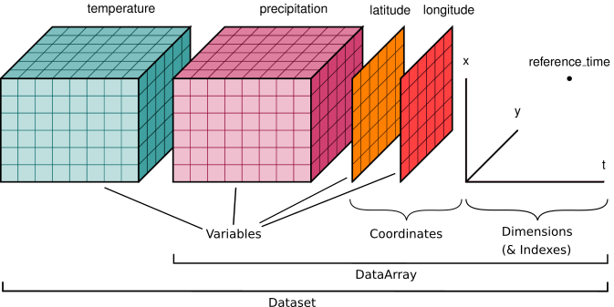
The Xarray Data Models#
“Xarray data models are borrowed from netCDF file format, which provides xarray with a natural and portable serialization format.”
—https://docs.xarray.dev/en/latest/getting-started-guide/why-xarray.html
``xarray.Dataset``
A dictionary-like container of DataArray objects with aligned dimensions
DataArray objects are classified as “coordinate variables” or “data variables”
All data variables have a shared union of coordinates
Serves a similar purpose to a
pandas.DataFrame
``xarray.DataArray``
A class that attaches dimension names, coordinates, and attributes to multi-dimensional arrays (aka “labeled arrays”)
An N-D generalization of a
pandas.Series
Exploring the Xarray Data Models#
The data used in this example can be found in the xcdat-data repository.
[1]:
# This style import is necessary to properly render Xarray's HTML output with
# the Jupyer RISE extension.
# GitHub Issue: https://github.com/damianavila/RISE/issues/594
# Source: https://github.com/smartass101/xarray-pydata-prague-2020/blob/main/rise.css

from IPython.core.display import HTML

style = """
<style>
.reveal pre.xr-text-repr-fallback {
    display: none;
}
.reveal ul.xr-sections {
    display: grid
}

.reveal ul ul.xr-var-list {
    display: contents
}
</style>
"""


HTML(style)
[1]:
[2]:
import xcdat as xc

ds = xc.tutorial.open_dataset("tas_amon_access")
/opt/miniconda3/envs/xcdat_notebook/lib/python3.13/site-packages/esmpy/interface/loadESMF.py:94: VersionWarning: ESMF installation version 8.8.0, ESMPy version 8.8.0b0
  warnings.warn("ESMF installation version {}, ESMPy version {}".format(
The Dataset Model#
[3]:
ds
[3]:
<xarray.Dataset> Size: 7MB
Dimensions:    (time: 60, bnds: 2, lat: 145, lon: 192)
Coordinates:
  * lat        (lat) float64 1kB -90.0 -88.75 -87.5 -86.25 ... 87.5 88.75 90.0
  * lon        (lon) float64 2kB 0.0 1.875 3.75 5.625 ... 354.4 356.2 358.1
    height     float64 8B 2.0
  * time       (time) object 480B 1870-01-16 12:00:00 ... 1874-12-16 12:00:00
Dimensions without coordinates: bnds
Data variables:
    time_bnds  (time, bnds) object 960B ...
    lat_bnds   (lat, bnds) float64 2kB ...
    lon_bnds   (lon, bnds) float64 3kB ...
    tas        (time, lat, lon) float32 7MB ...
Attributes: (12/48)
    Conventions:                     CF-1.7 CMIP-6.2
    activity_id:                     CMIP
    branch_method:                   standard
    branch_time_in_child:            0.0
    branch_time_in_parent:           87658.0
    creation_date:                   2020-06-05T04:06:11Z
    ...                              ...
    variant_label:                   r10i1p1f1
    version:                         v20200605
    license:                         CMIP6 model data produced by CSIRO is li...
    cmor_version:                    3.4.0
    tracking_id:                     hdl:21.14100/af78ae5e-f3a6-4e99-8cfe-5f2...
DODS_EXTRA.Unlimited_Dimension: timeA dictionary-like container of labeled arrays (DataArray objects) with aligned dimensions.
Key properties:
dims: a dictionary mapping from dimension names to the fixed length of each dimension (e.g., {‘x’: 6, ‘y’: 6, ‘time’: 8})coords: a dict-like container of DataArrays intended to label points used in ``data_vars`` (e.g., arrays of numbers, datetime objects or strings)data_vars: a dict-like container of DataArrays corresponding to variablesattrs: dict to hold arbitrary metadata
Source: https://docs.xarray.dev/en/stable/user-guide/data-structures.html#dataset
The DataArray Model#
[4]:
ds.tas
[4]:
<xarray.DataArray 'tas' (time: 60, lat: 145, lon: 192)> Size: 7MB
[1670400 values with dtype=float32]
Coordinates:
  * lat      (lat) float64 1kB -90.0 -88.75 -87.5 -86.25 ... 87.5 88.75 90.0
  * lon      (lon) float64 2kB 0.0 1.875 3.75 5.625 ... 352.5 354.4 356.2 358.1
    height   float64 8B 2.0
  * time     (time) object 480B 1870-01-16 12:00:00 ... 1874-12-16 12:00:00
Attributes:
    standard_name:  air_temperature
    long_name:      Near-Surface Air Temperature
    comment:        near-surface (usually, 2 meter) air temperature
    units:          K
    cell_methods:   area: time: mean
    cell_measures:  area: areacella
    history:        2020-06-05T04:06:10Z altered by CMOR: Treated scalar dime...
_ChunkSizes: [ 1 145 192]A class that attaches dimension names, coordinates, and attributes to multi-dimensional arrays (aka “labeled arrays”)
Key properties:
values: a numpy.ndarray holding the array’s valuesdims: dimension names for each axis (e.g., (‘x’, ‘y’, ‘z’))coords: a dict-like container of arrays (coordinates) that label each point (e.g., 1-dimensional arrays of numbers, datetime objects or strings)attrs: dict to hold arbitrary metadata (attributes)
Source: https://docs.xarray.dev/en/stable/user-guide/data-structures.html#dataarray
Resources for Learning Xarray#
Here are some highly recommended resources:
xCDAT Extends Xarray for Climate Data Analysis#
Some key xCDAT features are inspired by or ported from the core CDAT library
e.g., spatial averaging, temporal averaging, regrid2 for horizontal regridding
Other features leverage powerful libraries in the xarray ecosystem
xESMF for horizontal regridding
xgcm for vertical interpolation
CF-xarray for CF convention metadata interpretation
xCDAT strives to support datasets CF compliant and common non-CF compliant metadata (time units in “months since …” or “years since …”)
Inherent support for lazy operations and parallelism through xarray + dask


The Technical Design Philosophy#
Streamline the user experience of developing code to analyze climate data
Reduce the complexity and overhead for implementing certain features with xarray (e.g., temporal averaging, spatial averaging)
Encourage reusable functionalities through a single library
Leveraging the APIs#
xCDAT provides public APIs in two ways:
Top-level APIs functions
e.g.,
xcdat.open_dataset(),xcdat.center_times()Usually for opening datasets and performing dataset level operations
Accessor classes
xcdat provides
Datasetaccessors, which are implicit namespaces for custom functionality.Accessor namespaces clearly identifies separation from built-in xarray methods.
Operate on variables within the
xr.Datasete.g.,
ds.spatial,ds.temporal,ds.regridder

xcdat spatial functionality is exposed by chaining the .spatial accessor attribute to the xr.Dataset object.
Key Features in xCDAT#
Feature | API | Description |
Extend |
|
|
Temporal averaging |
|
|
Geospatial averaging |
|
|
Horizontal regridding |
|
|
Vertical regridding |
|
|
A Demo of xCDAT Capabilities#
Prerequisites
Installing
xcdatImport
xcdatOpen a dataset and apply postprocessing operations
Scenario 1 - Calculate the spatial averages over the tropical region
Scenario 2 - Calculate temporal average
Scenario 3 - Horizontal regridding (bilinear, gaussian grid)
Installing xcdat#
xCDAT is available on Anaconda under the conda-forge channel (https://anaconda.org/conda-forge/xcdat)
Two ways to install xcdat with recommended dependencies (xesmf):
Create a conda environment from scratch (
conda create)conda create -n <ENV_NAME> -c conda-forge xcdat conda activate <ENV_NAME>
Install
xcdatin an existing conda environment (conda install)conda activate <ENV_NAME> conda install -c conda-forge xcdat
Source: https://xcdat.readthedocs.io/en/latest/getting-started.html
Open the example dataset#
[5]:
# This gives access to all xcdat public top-level APIs and accessor classes.
import xcdat as xc

# We import these packages specifically for plotting. It is not required to use xcdat.
import matplotlib.pyplot as plt

ds = xc.tutorial.open_dataset("tas_amon_access")

# Unit adjustment from Kelvin to Celcius.
ds["tas"] = ds.tas - 273.15
[6]:
ds
[6]:
<xarray.Dataset> Size: 7MB
Dimensions:    (time: 60, bnds: 2, lat: 145, lon: 192)
Coordinates:
  * lat        (lat) float64 1kB -90.0 -88.75 -87.5 -86.25 ... 87.5 88.75 90.0
  * lon        (lon) float64 2kB 0.0 1.875 3.75 5.625 ... 354.4 356.2 358.1
    height     float64 8B 2.0
  * time       (time) object 480B 1870-01-16 12:00:00 ... 1874-12-16 12:00:00
Dimensions without coordinates: bnds
Data variables:
    time_bnds  (time, bnds) object 960B ...
    lat_bnds   (lat, bnds) float64 2kB ...
    lon_bnds   (lon, bnds) float64 3kB ...
    tas        (time, lat, lon) float32 7MB -29.36 -29.36 ... -31.07 -31.07
Attributes: (12/48)
    Conventions:                     CF-1.7 CMIP-6.2
    activity_id:                     CMIP
    branch_method:                   standard
    branch_time_in_child:            0.0
    branch_time_in_parent:           87658.0
    creation_date:                   2020-06-05T04:06:11Z
    ...                              ...
    variant_label:                   r10i1p1f1
    version:                         v20200605
    license:                         CMIP6 model data produced by CSIRO is li...
    cmor_version:                    3.4.0
    tracking_id:                     hdl:21.14100/af78ae5e-f3a6-4e99-8cfe-5f2...
DODS_EXTRA.Unlimited_Dimension: timeScenario 1: Spatial Averaging#
Related accessor: ds.spatial
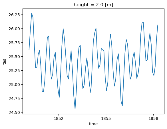
In this example, we calculate the spatial average of tas over the tropical region and plot the first 100 time steps.
[7]:
ds_trop_avg = ds.spatial.average("tas", axis=["X","Y"], lat_bounds=(-25,25))
ds_trop_avg.tas
[7]:
<xarray.DataArray 'tas' (time: 60)> Size: 480B
array([25.00067275, 25.30644298, 25.7617891 , 26.10626959, 26.01841282,
       25.5047623 , 25.28394064, 25.37295231, 25.72527095, 25.87376074,
       25.67985682, 25.22942709, 24.95699101, 25.48591822, 26.02279319,
       26.29556201, 26.18619426, 25.791096  , 25.50230606, 25.52068064,
       25.68326088, 25.78873469, 25.63775696, 25.15228934, 25.08228764,
       25.30220953, 25.69973578, 26.0328945 , 25.9973611 , 25.51339722,
       25.39540446, 25.45184812, 25.70660688, 25.75817938, 25.54315004,
       25.13706986, 24.96105631, 25.311973  , 25.7646741 , 26.01738372,
       26.01281503, 25.69728948, 25.3639977 , 25.5225464 , 25.77108789,
       25.84422784, 25.70096048, 25.11534178, 25.0415591 , 25.34789389,
       25.72121083, 25.91918215, 25.83924512, 25.55205376, 25.13493311,
       25.22239226, 25.43492285, 25.43073544, 25.26357054, 24.80680714])
Coordinates:
    height   float64 8B 2.0
* time (time) object 480B 1870-01-16 12:00:00 ... 1874-12-16 12:00:00[8]:
ds_trop_avg.tas.isel(time=slice(1, 100)).plot()
[8]:
[<matplotlib.lines.Line2D at 0x15f249a90>]
Scenario 2: Calculate temporal average#
Related accessor: ds.temporal
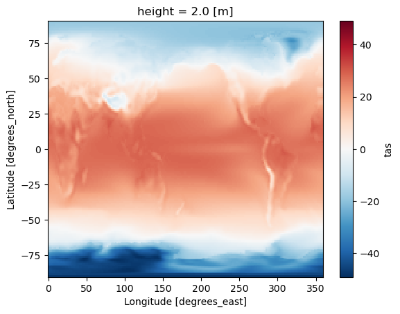
In this example, we calculate the temporal average of ``tas`` as a single snapshot (time dimension is collapsed).
[9]:
ds_avg = ds.temporal.average("tas", weighted=True)
ds_avg.tas
[9]:
<xarray.DataArray 'tas' (lat: 145, lon: 192)> Size: 223kB
array([[-48.33789281, -48.33789281, -48.33789281, ..., -48.33789281,
        -48.33789281, -48.33789281],
       [-45.11841101, -45.15598013, -45.19300779, ..., -45.00752255,
        -45.04406075, -45.08005955],
       [-44.16135662, -44.27207786, -44.3812548 , ..., -43.8142947 ,
        -43.93083878, -44.04664427],
       ...,
       [-18.87074617, -18.84301489, -18.81438219, ..., -18.96065605,
        -18.92790196, -18.89991471],
       [-18.98835924, -18.97666923, -18.96525417, ..., -19.02792192,
        -19.01732752, -19.00373892],
       [-19.36861239, -19.36861239, -19.36861239, ..., -19.36861239,
        -19.36861239, -19.36861239]])
Coordinates:
  * lat      (lat) float64 1kB -90.0 -88.75 -87.5 -86.25 ... 87.5 88.75 90.0
  * lon      (lon) float64 2kB 0.0 1.875 3.75 5.625 ... 352.5 354.4 356.2 358.1
    height   float64 8B 2.0
Attributes:
    operation:  temporal_avg
    mode:       average
    freq:       month
weighted: True[10]:
ds_avg.tas.plot(label="weighted")
[10]:
<matplotlib.collections.QuadMesh at 0x15f23d6a0>
Scenario 3: Horizontal Regridding#
Related accessor: ds.regridder
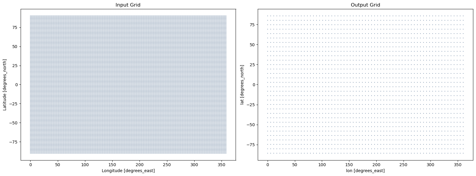
In this example, we will generate a gaussian grid with 32 latitudes to regrid our input data to.
Create the output grid#
[11]:
output_grid = xc.create_gaussian_grid(32)
output_grid
[11]:
<xarray.Dataset> Size: 2kB
Dimensions:   (lon: 65, bnds: 2, lat: 32)
Coordinates:
  * lon       (lon) float64 520B 0.0 5.625 11.25 16.88 ... 348.8 354.4 360.0
  * lat       (lat) float64 256B 85.76 80.27 74.74 ... -74.74 -80.27 -85.76
Dimensions without coordinates: bnds
Data variables:
    lon_bnds  (lon, bnds) float64 1kB -2.812 2.812 2.812 ... 357.2 357.2 362.8
lat_bnds (lat, bnds) float64 512B 90.0 83.21 83.21 ... -83.21 -83.21 -90.0Plot the Input vs. Output Grid#
[12]:
fig, axes = plt.subplots(ncols=2, figsize=(16, 6))

input_grid = ds.regridder.grid
input_grid.plot.scatter(x='lon', y='lat', s=5, ax=axes[0], add_colorbar=False, cmap=plt.cm.RdBu)
axes[0].set_title('Input Grid')

output_grid.plot.scatter(x='lon', y='lat', s=5, ax=axes[1], add_colorbar=False, cmap=plt.cm.RdBu)
axes[1].set_title('Output Grid')

plt.tight_layout()
Regrid the data#
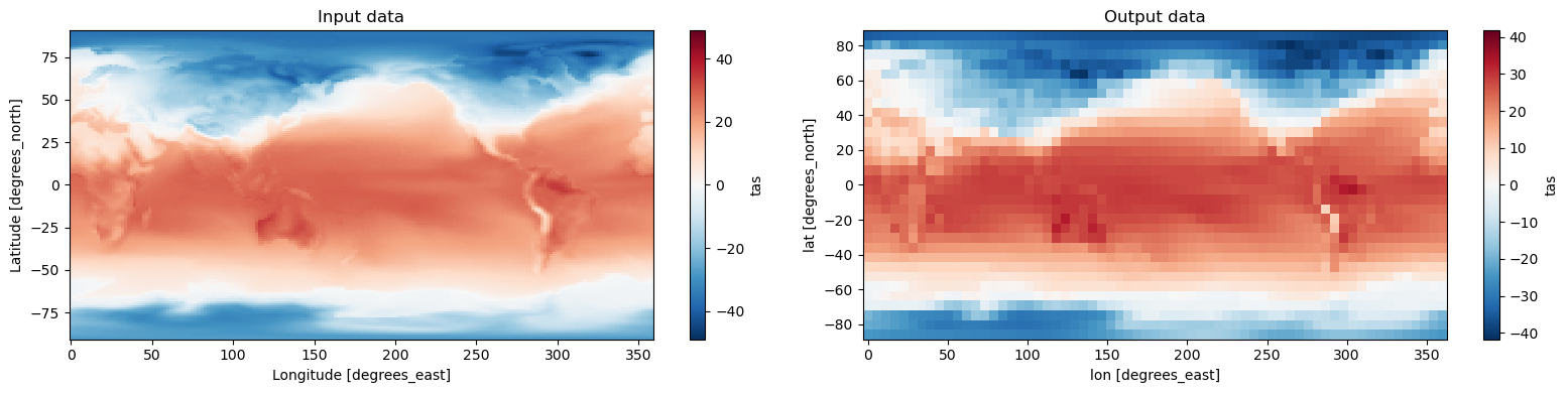
xCDAT offers horizontal regridding with xESMF (default) and a Python port of regrid2. We will be using xESMF to regrid.
[13]:
# xesmf supports "bilinear", "conservative", "nearest_s2d", "nearest_d2s", and "patch"
output = ds.regridder.horizontal('tas', output_grid, tool='xesmf', method='bilinear')
[14]:
fig, axes = plt.subplots(ncols=2, figsize=(16, 4))

ds.tas.isel(time=0).plot(ax=axes[0])
axes[0].set_title('Input data')

output.tas.isel(time=0).plot(ax=axes[1])
axes[1].set_title('Output data')

plt.tight_layout()
Parallelism with Dask#

Nearly all existing xarray methods have been extended to work automatically with Dask arrays for parallelism
—https://docs.xarray.dev/en/stable/user-guide/dask.html#using-dask-with-xarray
Parallelized xarray methods include indexing, computation, concatenating and grouped operations
xCDAT APIs that build upon xarray methods inherently support Dask parallelism
Dask arrays are loaded into memory only when absolutely required (e.g., generating weights for averaging)
[15]:
# Use .chunk() to activate Dask arrays
# NOTE: `open_mfdataset()` automatically chunks by the number of files, which
# might not be optimal.
ds = xc.tutorial.open_dataset("tas_amon_access", chunks={"time": "auto"})
ds
[15]:
<xarray.Dataset> Size: 7MB
Dimensions:    (time: 60, bnds: 2, lat: 145, lon: 192)
Coordinates:
  * lat        (lat) float64 1kB -90.0 -88.75 -87.5 -86.25 ... 87.5 88.75 90.0
  * lon        (lon) float64 2kB 0.0 1.875 3.75 5.625 ... 354.4 356.2 358.1
    height     float64 8B ...
  * time       (time) object 480B 1870-01-16 12:00:00 ... 1874-12-16 12:00:00
Dimensions without coordinates: bnds
Data variables:
    time_bnds  (time, bnds) object 960B dask.array<chunksize=(60, 2), meta=np.ndarray>
    lat_bnds   (lat, bnds) float64 2kB dask.array<chunksize=(145, 2), meta=np.ndarray>
    lon_bnds   (lon, bnds) float64 3kB dask.array<chunksize=(192, 2), meta=np.ndarray>
    tas        (time, lat, lon) float32 7MB dask.array<chunksize=(60, 145, 192), meta=np.ndarray>
Attributes: (12/48)
    Conventions:                     CF-1.7 CMIP-6.2
    activity_id:                     CMIP
    branch_method:                   standard
    branch_time_in_child:            0.0
    branch_time_in_parent:           87658.0
    creation_date:                   2020-06-05T04:06:11Z
    ...                              ...
    variant_label:                   r10i1p1f1
    version:                         v20200605
    license:                         CMIP6 model data produced by CSIRO is li...
    cmor_version:                    3.4.0
    tracking_id:                     hdl:21.14100/af78ae5e-f3a6-4e99-8cfe-5f2...
DODS_EXTRA.Unlimited_Dimension: timeFurther Dask Guidance#
Visit these pages for more guidance (e.g., when to parallelize):
Parallel computing with Dask (xCDAT): https://xcdat.readthedocs.io/en/latest/examples/parallel-computing-with-dask.html
Parallel computing with Dask (Xarray): https://docs.xarray.dev/en/stable/user-guide/dask.html
Xarray with Dask Arrays: https://examples.dask.org/xarray.html
Key Takeaways#
A driving need for a modern successor to CDAT
Serves the climate community in the long-term
xCDAT is an extension of xarray for climate data analysis on structured grids
Goal of providing features and utilities for simple and robust analysis of climate data
Where to Find xCDAT#
xCDAT is available for installation through Anaconda
Install command: ``conda install -c conda-forge xcdat xesmf``
Check out xCDAT’s Read the Docs, which we strive to keep up-to-date




Get Involved on GitHub!#
Code contributions are welcome and appreciated
GitHub Repository: xCDAT/xcdat
Contributing Guide: https://xcdat.readthedocs.io/en/latest/contributing.html
Submit and/or address tickets for feature suggestions, bugs, and documentation updates
GitHub Issues: xCDAT/xcdat#issues
Participate in forum discussions on version releases, architecture, feature suggestions, etc.
GitHub Discussions: xCDAT/xcdat#discussions