Horizontal Regridding#

Date: 09/26/22

Related APIs:

xarray.Dataset.regridder.horizontal

The data used in this example can be found through the Earth System Grid Federation (ESGF) search portal.

Overview#

We’ll cover horizontal regridding using the xESMF and Regrid2 tools as well as various methods supported by xESMF.

It should be noted that Regrid2 treats the grid cells as being flat.

Notebook Setup#

Create an Anaconda environment for this notebook using the command below, then select the kernel in Jupyter.

conda create -n xcdat_notebook -c conda-forge python xarray netcdf4 xcdat xesmf matplotlib nc-time-axis jupyter

xesmf is required for horizontal regridding with xESMF
matplotlib is an optional dependency required for plotting with xarray
nc-time-axis is an optional dependency required for matplotlib to plot cftime coordinates

[1]:

%matplotlib inline

import os
import sys
os.environ["ESMFMKFILE"] = sys.prefix + "/lib/esmf.mk" # TODO remove after esmf>=8.5
import xesmf

[2]:

import matplotlib.pyplot as plt
import xarray as xr
import xcdat

1. Open the Dataset#

We are using xarray’s OPeNDAP support to read a netCDF4 dataset file directly from its source. The data is not loaded over the network until we perform operations on it (e.g., temperature unit adjustment).

More information on the xarray’s OPeNDAP support can be found here.

[3]:

filepath = "http://aims3.llnl.gov/thredds/dodsC/css03_data/CMIP6/CMIP/CCCma/CanESM5/historical/r13i1p1f1/Amon/tas/gn/v20190429/tas_Amon_CanESM5_historical_r13i1p1f1_gn_185001-201412.nc"

ds = xcdat.open_dataset(filepath)

# Unit adjust (-273.15, K to C)
ds["tas"] = ds["tas"] - 273.15

ds

[3]:

<xarray.Dataset>
Dimensions:    (time: 1980, bnds: 2, lat: 64, lon: 128)
Coordinates:
  * time       (time) object 1850-01-16 12:00:00 ... 2014-12-16 12:00:00
  * lat        (lat) float64 -87.86 -85.1 -82.31 -79.53 ... 82.31 85.1 87.86
  * lon        (lon) float64 0.0 2.812 5.625 8.438 ... 348.8 351.6 354.4 357.2
    height     float64 2.0
Dimensions without coordinates: bnds
Data variables:
    time_bnds  (time, bnds) object ...
    lat_bnds   (lat, bnds) float64 ...
    lon_bnds   (lon, bnds) float64 ...
    tas        (time, lat, lon) float32 -25.04 -25.28 -25.49 ... -25.93 -25.73
Attributes: (12/54)
    CCCma_model_hash:                7e8e715f3f2ce47e1bab830db971c362ca329419
    CCCma_parent_runid:              rc3.1-pictrl
    CCCma_pycmor_hash:               33c30511acc319a98240633965a04ca99c26427e
    CCCma_runid:                     rc3.1-his13
    Conventions:                     CF-1.7 CMIP-6.2
    YMDH_branch_time_in_child:       1850:01:01:00
    ...                              ...
    variable_id:                     tas
    variant_label:                   r13i1p1f1
    version:                         v20190429
    license:                         CMIP6 model data produced by The Governm...
    cmor_version:                    3.4.0
    DODS_EXTRA.Unlimited_Dimension:  time

2. Create the output grid#

Related API: xcdat.create_gaussian_grid()

In this example, we will generate a gaussian grid with 32 latitudes to regrid our input data to.

Alternatively a grid can be loaded from a file, e.g.

grid_urlpath = "http://aims3.llnl.gov/thredds/dodsC/css03_data/CMIP6/CMIP/NOAA-GFDL/GFDL-CM4/abrupt-4xCO2/r1i1p1f1/day/tas/gr2/v20180701/tas_day_GFDL-CM4_abrupt-4xCO2_r1i1p1f1_gr2_00010101-00201231.nc"

grid_ds = xcdat.open_dataset(grid_urlpath)

output_grid = grid_ds.regridder.grid

Other related APIs available for creating grids: xcdat.create_grid() and xcdat.create_uniform_grid()

[4]:

output_grid = xcdat.create_gaussian_grid(32)

fig, axes = plt.subplots(ncols=2, figsize=(16, 4))

ds.regridder.grid.plot.scatter(x="lon", y="lat", s=4, ax=axes[0])
axes[0].set_title("Input Grid")

output_grid.plot.scatter(x="lon", y="lat", s=4, ax=axes[1])
axes[1].set_title("Output Grid")

plt.tight_layout()

../_images/examples_regridding-horizontal_7_0.png

3. Regrid the data#

Here we will regrid the input data to the ouptut grid using the xESMF tool and the bilinear method.

[5]:

output = ds.regridder.horizontal("tas", output_grid, tool="xesmf", method="bilinear")

fig, axes = plt.subplots(ncols=2, figsize=(16, 4))

ds.tas.isel(time=0).plot(ax=axes[0], vmin=-40, vmax=40, extend='both', cmap = 'RdBu_r')
axes[0].set_title("Input data")

output.tas.isel(time=0).plot(ax=axes[1], vmin=-40, vmax=40, extend='both', cmap = 'RdBu_r')
axes[1].set_title("Output data")

plt.tight_layout()

../_images/examples_regridding-horizontal_9_0.png

4. Regridding algorithms#

In this example, we will compare the different regridding methods supported by xESMF.

You can find a more in depth comparison on xESMF’s documentation.

Methods:

bilinear
conservative
nearest_s2d
nearest_d2s
patch

[6]:

methods = ["bilinear", "conservative", "nearest_s2d", "nearest_d2s", "patch"]

fig, axes = plt.subplots(3, 2, figsize=(16, 12))

axes = axes.flatten()

for i, method in enumerate(methods):
    output = ds.regridder.horizontal("tas", output_grid, tool="xesmf", method=method)

    output.tas.isel(time=0).plot(ax=axes[i], vmin=-40, vmax=40, extend='both', cmap = 'RdBu_r')

    axes[i].set_title(method)

axes[-1].set_visible(False)

plt.tight_layout()

../_images/examples_regridding-horizontal_11_0.png

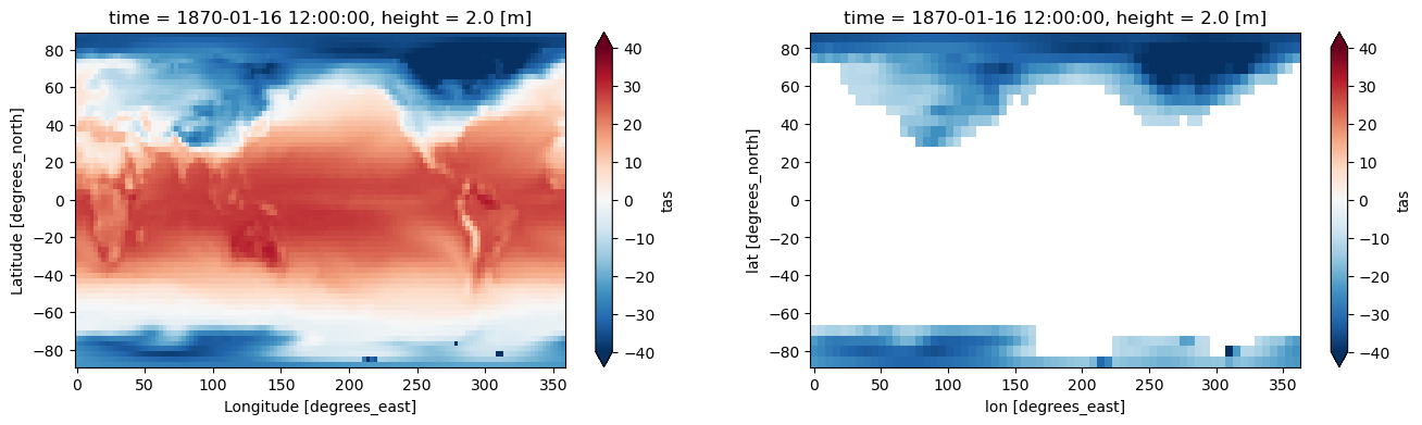
5. Masking#

xESMF supports masking by simply adding a data variable with the id mask.

See xESMF documentation for additonal details.

[7]:

ds["mask"] = xr.where(ds.tas.isel(time=0) < -10, 1, 0)

masked_output = ds.regridder.horizontal(
    "tas", output_grid, tool="xesmf", method="bilinear"
)

fig, axes = plt.subplots(ncols=2, figsize=(18, 4))

ds["mask"].plot(ax=axes[0], cmap="binary_r")
axes[0].set_title("Mask")

masked_output.tas.isel(time=0).plot(ax=axes[1], vmin=-40, vmax=40, extend='both', cmap='RdBu_r')
axes[1].set_title("Masked output")

plt.tight_layout()

../_images/examples_regridding-horizontal_13_0.png

6. Regridding using `regrid2`#

Regrid2 is a conservative regridder for rectilinear (lat/lon) grids originally from the cdutil package from CDAT.

This regridder assumes constant latitude lines when generating weights.

[8]:

output = ds.regridder.horizontal("tas", output_grid, tool="regrid2")

fig, axes = plt.subplots(ncols=2, figsize=(16, 4))

ds.tas.isel(time=0).plot(ax=axes[0], vmin=-40, vmax=40, extend='both', cmap = 'RdBu_r')

output.tas.isel(time=0).plot(ax=axes[1], vmin=-40, vmax=40, extend='both', cmap = 'RdBu_r')

[8]:

<matplotlib.collections.QuadMesh at 0x7ff3d84aa890>

../_images/examples_regridding-horizontal_15_1.png

Horizontal Regridding

Contents