Vertical Regridding#
Authors: Jason Boutte and Jill Zhang
Updated: 11/07/24 [xcdat v0.8.0]
Related APIs:
We’ll cover vertical regridding using xgcm. Two examples are outlined here to apply vertical regridding/remapping using ocean variables and atmosphere variables, respectively.
The data used in this example can be found in the xcdat-data repository.
Notebook Kernel Setup#
Users can install their own instance of xcdat and follow these examples using their own environment (e.g., with VS Code, Jupyter, Spyder, iPython) or enable xcdat with existing JupyterHub instances.
First, create the conda environment:
conda create -n xcdat_notebook -c conda-forge xcdat xesmf matplotlib ipython ipykernel cartopy nc-time-axis gsw-xarray jupyter pooch
Then install the kernel from the xcdat_notebook environment using ipykernel and name the kernel with the display name (e.g., xcdat_notebook):
python -m ipykernel install --user --name xcdat_notebook --display-name xcdat_notebook
Then to select the kernel xcdat_notebook in Jupyter to use this kernel.
Example 1: Remapping Ocean Variables#
[1]:
%matplotlib inline

import dask.array as da
import gsw_xarray as gsw
import matplotlib.pyplot as plt
import numpy as np
import pandas as pd
import xarray as xr
import xcdat as xc

import warnings

warnings.filterwarnings("ignore")
/opt/miniconda3/envs/xcdat_notebook/lib/python3.13/site-packages/esmpy/interface/loadESMF.py:94: VersionWarning: ESMF installation version 8.8.0, ESMPy version 8.8.0b0
  warnings.warn("ESMF installation version {}, ESMPy version {}".format(
[2]:
# Keys for sea water potential temperature (thetao) and salinity (so) from the NCAR model in CMIP6
keys = ["so_omon_cesm2", "thetao_omon_cesm2"]

ds = xr.merge([xc.tutorial.open_dataset(x) for x in keys])

# lev coordinate is in cm and bounds is in m, convert lev to m
with xr.set_options(keep_attrs=True):
    ds.lev.load()
    ds["lev"] = ds.lev / 100
    ds.lev.attrs["units"] = "meters"

ds = ds.drop_vars(["nlon_bnds"])
ds
2025-03-14 17:03:48,385 [WARNING]: bounds.py(add_missing_bounds:194) >> The nlat coord variable has a 'units' attribute that is not in degrees.
2025-03-14 17:03:48,385 [WARNING]: bounds.py(add_missing_bounds:194) >> The nlat coord variable has a 'units' attribute that is not in degrees.
2025-03-14 17:03:48,412 [WARNING]: bounds.py(add_missing_bounds:194) >> The nlat coord variable has a 'units' attribute that is not in degrees.
2025-03-14 17:03:48,412 [WARNING]: bounds.py(add_missing_bounds:194) >> The nlat coord variable has a 'units' attribute that is not in degrees.
[2]:
<xarray.Dataset> Size: 183MB
Dimensions:    (time: 3, lev: 60, nlat: 384, nlon: 320, d2: 2, vertices: 4)
Coordinates:
    lat        (nlat, nlon) float64 983kB -79.22 -79.22 -79.22 ... 72.19 72.19
  * lev        (lev) float64 480B 5.0 15.0 25.0 ... 5.125e+03 5.375e+03
    lon        (nlat, nlon) float64 983kB 320.6 321.7 322.8 ... 319.4 319.8
  * nlat       (nlat) int32 2kB 1 2 3 4 5 6 7 8 ... 378 379 380 381 382 383 384
  * nlon       (nlon) int32 1kB 1 2 3 4 5 6 7 8 ... 314 315 316 317 318 319 320
  * time       (time) object 24B 1850-01-15 13:00:00.000008 ... 1850-03-15 12...
Dimensions without coordinates: d2, vertices
Data variables:
    so         (time, lev, nlat, nlon) float32 88MB ...
    time_bnds  (time, d2) object 48B 1850-01-01 02:00:00 ... 1850-04-01 00:00:00
    lat_bnds   (nlat, nlon, vertices) float32 2MB -79.49 -79.49 ... 72.41 72.41
    lon_bnds   (nlat, nlon, vertices) float32 2MB 320.0 321.1 ... 320.0 319.6
    lev_bnds   (lev, d2) float32 480B 0.0 10.0 10.0 ... 5.25e+03 5.5e+03
    thetao     (time, lev, nlat, nlon) float32 88MB ...
Attributes: (12/45)
    Conventions:            CF-1.7 CMIP-6.2
    activity_id:            CMIP
    case_id:                15
    cesm_casename:          b.e21.BHIST.f09_g17.CMIP6-historical.001
    contact:                cesm_cmip6@ucar.edu
    creation_date:          2019-01-16T23:15:40Z
    ...                     ...
    sub_experiment:         none
    sub_experiment_id:      none
    branch_time_in_parent:  219000.0
    branch_time_in_child:   674885.0
    branch_method:          standard
further_info_url: https://furtherinfo.es-doc.org/CMIP6.NCAR.CESM2.h...2. Create the output grid#
Related API: xc.create_grid()
In this example, we will generate a vertical grid with a linear spaced level coordinate using xc.create_grid
Alternatively a grid can be loaded from a file, e.g.
grid_urlpath = "http://aims3.llnl.gov/thredds/dodsC/css03_data/CMIP6/CMIP/NOAA-GFDL/GFDL-CM4/abrupt-4xCO2/r1i1p1f1/day/tas/gr2/v20180701/tas_day_GFDL-CM4_abrupt-4xCO2_r1i1p1f1_gr2_00010101-00201231.nc"

grid_ds = xc.open_dataset(grid_urlpath)

output_grid = grid_ds.regridder.grid
[3]:
output_grid = xc.create_grid(z=xc.create_axis("lev", np.linspace(5, 537, 10)))

output_grid
[3]:
<xarray.Dataset> Size: 240B
Dimensions:   (lev: 10, bnds: 2)
Coordinates:
  * lev       (lev) float64 80B 5.0 64.11 123.2 182.3 ... 418.8 477.9 537.0
Dimensions without coordinates: bnds
Data variables:
lev_bnds (lev, bnds) float64 160B -24.56 34.56 34.56 ... 507.4 507.4 566.63. Regridding using the linear method#
Related API: xarray.Dataset.regridder.vertical()
Here we will regrid the input data to the output grid using the xgcm tool and the linear method.
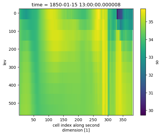
We’ll interpolate salinity onto the new vertical grid.
[4]:
output = ds.regridder.vertical("so", output_grid, tool="xgcm", method="linear")

output.so.isel(time=0).mean(dim="nlon").plot()
plt.gca().invert_yaxis()
2025-03-14 17:03:48,544 [WARNING]: bounds.py(add_missing_bounds:194) >> The nlat coord variable has a 'units' attribute that is not in degrees.
2025-03-14 17:03:48,544 [WARNING]: bounds.py(add_missing_bounds:194) >> The nlat coord variable has a 'units' attribute that is not in degrees.
4. Regridding from depth to density space#
Related API: xarray.Dataset.regridder.vertical()
Here we will regrid the input data to the output grid using the xgcm tool and the linear method.
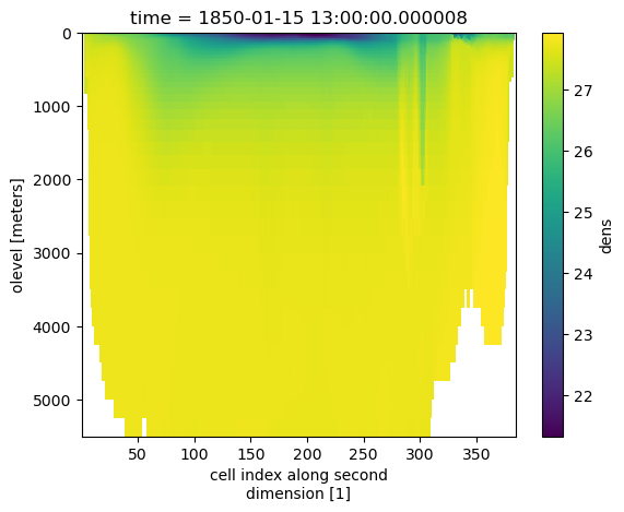
We’ll remap salinity into density space.
[5]:
# Apply gsw function to calculate potential density from potential temperature (thetao) and salinity (so)
ds["dens"] = gsw.sigma0(ds.so, ds.thetao)

ds.dens.isel(time=0).mean(dim="nlon").plot()
plt.gca().invert_yaxis()
[6]:
density_grid = xc.create_grid(z=xc.create_axis("lev", np.linspace(6, 26, 40)))

output = ds.regridder.vertical(
    "so", density_grid, tool="xgcm", method="linear", target_data="dens"
)

output.so.isel(time=0).mean(dim="nlon").plot()
plt.gca().invert_yaxis()
2025-03-14 17:03:50,272 [WARNING]: bounds.py(add_missing_bounds:194) >> The nlat coord variable has a 'units' attribute that is not in degrees.
2025-03-14 17:03:50,272 [WARNING]: bounds.py(add_missing_bounds:194) >> The nlat coord variable has a 'units' attribute that is not in degrees.
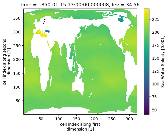
5. Regridding using the conservative method#
Related API: xarray.Dataset.regridder.vertical()
Here we will regrid the input data to the output grid using the xgcm tool and the conservative method.
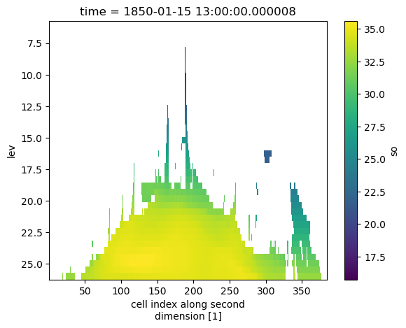
We’ll transform model levels using conservative regridding. In order to perform the regridding we’ll need two grid positions, the lev coordinate is center and we”ll create the outer points using cf_xarray”s bounds_to_vertices.
[7]:
ds_olev = ds.cf.bounds_to_vertices("lev").rename({"lev_vertices": "olev"})

output = ds_olev.regridder.vertical(
    "so",
    output_grid,
    tool="xgcm",
    method="conservative",
    grid_positions={"center": "lev", "outer": "olev"},
)

output.so.isel(time=0).sel(lev=0, method="nearest").plot()
2025-03-14 17:03:51,436 [WARNING]: bounds.py(add_missing_bounds:194) >> The nlat coord variable has a 'units' attribute that is not in degrees.
2025-03-14 17:03:51,436 [WARNING]: bounds.py(add_missing_bounds:194) >> The nlat coord variable has a 'units' attribute that is not in degrees.
[7]:
<matplotlib.collections.QuadMesh at 0x1773b6e90>
Example 2: Remapping Atmosphere Variables#
1. Open dataset#
For this example, we are using monthly cloud fraction data and monthly air temperature data from the E3SM-2.0 model.
[8]:
ds_ta = xc.tutorial.open_dataset("ta_amon_e3sm2", add_bounds=["Z"])
ds_cl = xc.tutorial.open_dataset("cl_amon_e3sm2")
[9]:
ds_ta
[9]:
<xarray.Dataset> Size: 15MB
Dimensions:    (time: 3, bnds: 2, plev: 19, lat: 180, lon: 360)
Coordinates:
  * plev       (plev) float64 152B 1e+05 9.25e+04 8.5e+04 ... 1e+03 500.0 100.0
  * lat        (lat) float64 1kB -89.5 -88.5 -87.5 -86.5 ... 86.5 87.5 88.5 89.5
  * lon        (lon) float64 3kB 0.5 1.5 2.5 3.5 4.5 ... 356.5 357.5 358.5 359.5
  * time       (time) object 24B 1850-01-16 12:00:00 ... 1850-03-16 12:00:00
Dimensions without coordinates: bnds
Data variables:
    time_bnds  (time, bnds) object 48B ...
    lat_bnds   (lat, bnds) float64 3kB ...
    lon_bnds   (lon, bnds) float64 6kB ...
    ta         (time, plev, lat, lon) float32 15MB ...
    plev_bnds  (plev, bnds) float64 304B 1.038e+05 9.625e+04 ... 300.0 -100.0
Attributes: (12/49)
    Conventions:                     CF-1.7 CMIP-6.2
    activity_id:                     CMIP
    branch_method:                   standard
    branch_time_in_child:            0.0
    branch_time_in_parent:           36500.0
    creation_date:                   2022-08-31T00:29:52Z
    ...                              ...
    license:                         CMIP6 model data produced by E3SM-Projec...
    cmor_version:                    3.6.1
    tracking_id:                     hdl:21.14100/6e383052-7075-49db-a426-67d...
    version:                         v20220830
    references:                      Golaz, J.-C., L. P. Van Roekel, X. Zheng...
DODS_EXTRA.Unlimited_Dimension: time2. Create the output grid#
Related API: xc.create_grid()
In this example, we will generate a grid with a linear spaced level coordinate.
[10]:
output_grid = xc.create_grid(z=xc.create_axis("lev", np.linspace(100000, 1, 13)))

output_grid
[10]:
<xarray.Dataset> Size: 312B
Dimensions:   (lev: 13, bnds: 2)
Coordinates:
  * lev       (lev) float64 104B 1e+05 9.167e+04 8.333e+04 ... 8.334e+03 1.0
Dimensions without coordinates: bnds
Data variables: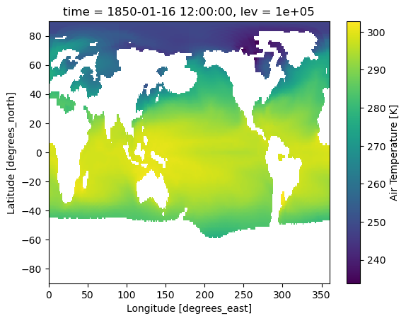
lev_bnds (lev, bnds) float64 208B 1.042e+05 9.583e+04 ... -4.166e+033. Remapping air temperature on pressure levels to a set of target pressure levels.#
Related API: xarray.Dataset.regridder.vertical()
Here we will regrid the input data to the output grid using the xgcm tool and the log method.
We’ll remap pressure levels.
[11]:
# Remap from original pressure level to target pressure level using logarithmic interpolation
# Note: output grids can be either ascending or descending
output_ta = ds_ta.regridder.vertical("ta", output_grid, method="log")

output_ta.ta.isel(time=0, lev=0).plot()
[11]:
<matplotlib.collections.QuadMesh at 0x175eab250>
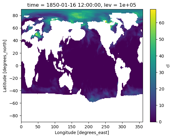
4: Remap cloud fraction from model hybrid coordinate to pressure levels#
Related API: xarray.Dataset.regridder.vertical()
Here we will regrid the input data to the output grid using the xgcm tool and the linear method.
We’ll remap cloud fraction into pressure space.
[12]:
# Build hybrid pressure coordinate
def hybrid_coordinate(p0, a, b, ps, **kwargs):
    return a * p0 + b * ps


pressure = hybrid_coordinate(**ds_cl.data_vars)

pressure
[12]:
<xarray.DataArray (lev: 72, time: 3, lat: 180, lon: 360)> Size: 112MB
array([[[[6.85818450e+04, 6.85818450e+04, 6.85818450e+04, ...,
          7.05259253e+04, 7.05259253e+04, 7.05259253e+04],
         [6.92225598e+04, 6.92220606e+04, 6.92210543e+04, ...,
          7.13934393e+04, 7.13948044e+04, 7.13954831e+04],
         [6.96804641e+04, 6.96804641e+04, 6.96804641e+04, ...,
          7.20169379e+04, 7.20169379e+04, 7.20169379e+04],
         ...,
         [1.01909534e+05, 1.01909534e+05, 1.01909534e+05, ...,
          1.01960629e+05, 1.01960629e+05, 1.01960629e+05],
         [1.01971028e+05, 1.01971098e+05, 1.01971230e+05, ...,
          1.02018331e+05, 1.02018207e+05, 1.02018144e+05],
         [1.02057070e+05, 1.02057070e+05, 1.02057070e+05, ...,
          1.02098617e+05, 1.02098617e+05, 1.02098617e+05]],

        [[6.85818450e+04, 6.85818450e+04, 6.85818450e+04, ...,
          7.05259253e+04, 7.05259253e+04, 7.05259253e+04],
         [6.92225598e+04, 6.92220606e+04, 6.92210543e+04, ...,
          7.13934393e+04, 7.13948044e+04, 7.13954831e+04],
         [6.96804641e+04, 6.96804641e+04, 6.96804641e+04, ...,
          7.20169379e+04, 7.20169379e+04, 7.20169379e+04],
...
         [1.23825413e+01, 1.23825413e+01, 1.23825413e+01, ...,
          1.23825413e+01, 1.23825413e+01, 1.23825413e+01],
         [1.23825413e+01, 1.23825413e+01, 1.23825413e+01, ...,
          1.23825413e+01, 1.23825413e+01, 1.23825413e+01],
         [1.23825413e+01, 1.23825413e+01, 1.23825413e+01, ...,
          1.23825413e+01, 1.23825413e+01, 1.23825413e+01]],

        [[1.23825413e+01, 1.23825413e+01, 1.23825413e+01, ...,
          1.23825413e+01, 1.23825413e+01, 1.23825413e+01],
         [1.23825413e+01, 1.23825413e+01, 1.23825413e+01, ...,
          1.23825413e+01, 1.23825413e+01, 1.23825413e+01],
         [1.23825413e+01, 1.23825413e+01, 1.23825413e+01, ...,
          1.23825413e+01, 1.23825413e+01, 1.23825413e+01],
         ...,
         [1.23825413e+01, 1.23825413e+01, 1.23825413e+01, ...,
          1.23825413e+01, 1.23825413e+01, 1.23825413e+01],
         [1.23825413e+01, 1.23825413e+01, 1.23825413e+01, ...,
          1.23825413e+01, 1.23825413e+01, 1.23825413e+01],
         [1.23825413e+01, 1.23825413e+01, 1.23825413e+01, ...,
          1.23825413e+01, 1.23825413e+01, 1.23825413e+01]]]])
Coordinates:
  * lev      (lev) float64 576B 0.9985 0.9938 0.9862 ... 0.0001828 0.0001238
  * lat      (lat) float64 1kB -89.5 -88.5 -87.5 -86.5 ... 86.5 87.5 88.5 89.5
  * lon      (lon) float64 3kB 0.5 1.5 2.5 3.5 4.5 ... 356.5 357.5 358.5 359.5
* time (time) object 24B 1850-01-16 12:00:00 ... 1850-03-16 12:00:00[13]:
new_pressure_grid = xc.create_grid(
    z=xc.create_axis("lev", np.linspace(100000, 1, 13))
)

output_cl = ds_cl.regridder.vertical(
    "cl", new_pressure_grid, method="linear", target_data=pressure
)

output_cl.cl.isel(time=0, lev=0).plot()
[13]:
<matplotlib.collections.QuadMesh at 0x17f0f9e50>
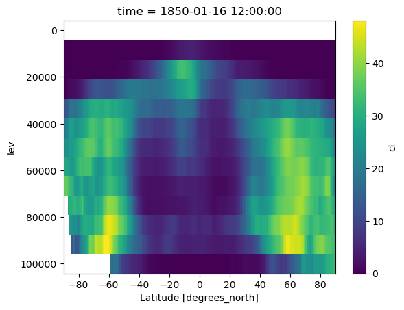
[14]:
output_cl.cl.isel(time=0).mean(dim="lon").plot()
plt.gca().invert_yaxis()